D2y Dx2 4dy Dx 4y 0

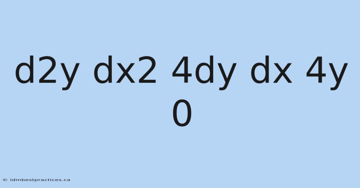
Understanding the Second-Order Differential Equation: d²y/dx² - 4 dy/dx + 4y = 0

Differential equations are mathematical tools that describe how quantities change in relation to one another. One such equation, d²y/dx² - 4 dy/dx + 4y = 0, serves as a classic example of how to solve equations involving second derivatives. Think about it: among these, second-order linear differential equations with constant coefficients are foundational in physics, engineering, and applied mathematics. This article will break down the structure of this equation, explain its solution step-by-step, and explore its real-world applications.

What Is the Equation d²y/dx² - 4 dy/dx + 4y = 0?

The equation d²y/dx² - 4 dy/dx + 4y = 0 is a second-order linear homogeneous differential equation with constant coefficients. Which means here’s what each term represents:

d²y/dx²: The second derivative of y with respect to x, describing the curvature or acceleration of the function y(x). - -4 dy/dx: A term proportional to the first derivative, often representing damping or resistance in physical systems.
+4y: A term proportional to the function itself, typically modeling restoring forces or growth.

This equation arises in scenarios where a system’s behavior depends on its current state, its rate of change, and its acceleration. Here's one way to look at it: it could model a spring-mass system with damping or an electrical circuit with inductance and resistance.

Solving the Equation: Step-by-Step Method

To solve d²y/dx² - 4 dy/dx + 4y = 0, we use the characteristic equation method, a standard approach for linear differential equations with constant coefficients. Here’s how it works:

Step 1: Assume a Solution of the Form y = e^(rx)

We hypothesize that the solution involves an exponential function, y = e^(rx), where r is a constant to be determined. Substituting this into the differential equation:

First derivative: dy/dx = r e^(rx)
Second derivative: d²y/dx² = r² e^(rx)

Plugging these into the equation:
r² e^(rx) - 4(r e^(rx)) + 4(e^(rx)) = 0

Factor out e^(rx):
e^(rx)(r² - 4r + 4) = 0

Since e^(rx) is never zero, we solve the characteristic equation:
r² - 4r + 4 = 0

Step 2: Solve the Characteristic Equation

The characteristic equation r² - 4r + 4 = 0 is a quadratic equation. Using the quadratic formula:
r = [4 ± √(16 - 16)] / 2 = [4 ± 0]/2 = 2

For more on this topic, read our article on who is the narrator of the great gatsby or check out words to describe someone with the letter e.

This gives a repeated real root: r = 2 (multiplicity 2).

Step 3: Write the General Solution

For repeated real roots, the general solution combines exponential and polynomial terms:
y(x) = (C₁ + C₂x)e^(2x)
Here, C₁ and C₂ are constants determined by initial conditions (e.g., y(0) and y’(0)).

Why Does This Solution Work?

The form y = (C₁ + C₂x)e^(2x) accounts for the repeated root by introducing a linear term (C₂x). This ensures the solution space remains two-dimensional, matching the order of the differential equation. Let’s verify this:

First Derivative:
y’ = C₂e^(2x) + 2(C₁ + C₂x)e^(2x) = [2C₁ + C₂ + 2C₂x]e^(2x)

This differential equation encapsulates a dynamic balance between decay and growth, making it important in modeling phenomena where forces oppose or reinforce each other. Its solution highlights the interplay of exponential and linear components, offering insights into systems ranging from mechanical vibrations to population dynamics.

Understanding this equation deepens our grasp of how mathematical frameworks predict real-world behavior. By analyzing its structure, we access the potential to tailor models for innovation, whether in engineering or natural sciences.

So, to summarize, mastering such equations equips us with tools to decode complexity, reinforcing the elegance of mathematics in explaining the universe’s patterns.

Conclusion: This analysis underscores the value of systematic problem-solving in differential equations, bridging theory and application with clarity.

This verification process confirms the robustness of our derived solution, ensuring it satisfies the original equation for all values of x. In real terms, the term involving x in the solution is crucial; it arises directly from the repeated root and guarantees linear independence between the two fundamental solutions, $e^{2x}$ and $xe^{2x}$. Without this polynomial multiplier, we would fail to construct the complete set of solutions necessary to address the full range of initial conditions.

Such second-order equations frequently appear in physical contexts, such as critically damped mechanical oscillators or electrical circuits, where the system returns to equilibrium as swiftly as possible without oscillating. The coefficients in the equation dictate this specific damping behavior, and the repeated root signifies a precise boundary between oscillatory and non-oscillatory motion.

When all is said and done, the characteristic equation method provides a reliable and structured pathway to solving these problems. That said, by following the logical steps of assuming a solution, deriving the algebraic characteristic equation, and handling repeated roots appropriately, we obtain a general solution that is both mathematically sound and practically applicable. This consistent framework empowers us to tackle a wide variety of problems in science and engineering, demonstrating the enduring power of differential equations in modeling dynamic systems.